Advisor Perspectives welcomes guest contributions. The views presented here do not necessarily represent those of Advisor Perspectives.
Q1 hedge fund letters, conference, scoops etc

The seasonal effect, namely that equities do better from November through April, is well-known. This article provides a rigorous statistical test of the effect and a trading strategy that profits from it.
My long-term study supporting this observation can be found here. A related switching strategy model with cyclical and defensive ETFs is described here.
The seasonality of the S&P 500 is easily verified. The S&P 500 with dividends from 1960 onward returned on average 1.92% for the six-month periods May through October, the “bad-period.” For the other six months, the “good-period,” from November through April, the average return was 8.47%.
Visually observing is not an adequate way to assess effectiveness. It is more rigorous – but nonetheless quite easy – to statistically demonstrate that the six months from November to April are usually good-periods for equities. The null hypothesis H0 is the default position, namely that there is no difference between the average returns of the good-periods and bad-periods, the average return hereinafter referred to as the “H0-return”.
Quantifying stock market seasonality with likelihood ratios
In evidence-based medicine, likelihood ratios assess the reliability of a diagnostic test, leading to improved patient outcomes and refined drug regimens. In finance, likelihood ratios can quantify the reliability of a financial test as well. For example, one can check the dependability of a recession indicator, as described here.
In medicine, likelihood ratios estimate how much the probability that a patient has a particular disease changes from before a diagnostic test is given to after its result is known. One can use the same concept to determine the probability of stock market performance over a particular period in the year when the outcome of a relevant indicator’s test is positive or negative.
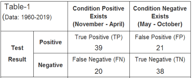
The time over which I tested this is from January 1960 to April 2019, consisting of 59 cyclical good-periods (condition positive) and 59 cyclical bad-periods (condition negative) for stocks, totaling 118 six-month periods, and showing an average return of 5.20% for all periods, the H0-return.
An indicator can be sending one of the following four messages, depending on the actual return for a period and its magnitude relative to the H0-return. For the condition positive the possibilities are:
- a correct call that the return for the good-period is greater than the H0-return (true positive, TP); or
- a false call (false positive, FP) when the return for the good-period is less than the H0-return.
For the condition negative the possibilities are:
- a valid negative call that the return for the bad-period is less than the H0-return (true negative, TN); or
- a wrong negative call (false negative, FN) when return for the bad-period is greater than the H0-return.
How often one of those conditions occurs over the observation period are the raw data for the analysis, shown in the Table-1 for my specific investigation.
Read the full article here by Georg Vrba, Advisor Perspectives


